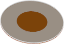
Circular patch antenna
The present example considers a circular patch antenna.
Circular patch antenna.
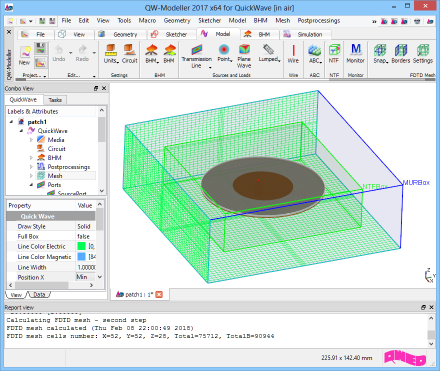
Circular patch antenna project in QW-Modeller.
Geometry of the antenna consists of circular base with diameter of 86 mm and 1 mm height made of PEC, circular dielectric plate with height of 0.787 mm and diameter of 86mm made of teflon, and infinitely thin (0 mm in thickness) circular patch of 42 mm in diameter.
The model is surrounded by superabsorbing (MUR) box.
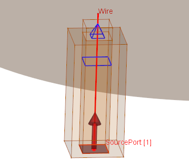
In practical designs it often happens that a patch antenna is fed with a vertical coaxial line. Such a line may have a very small diameter, when compared to the dimensions of the patch and to the considered wavelengths. In such a case it would be impractical to mesh the cross-section of the line into sufficiently small FDTD cells reproducing accurately the cylindrical shape of the conductors. This would unnecessarily provoke a drastic increase in the overall computing time of the project.
Thus in this example a different approach is used. The cross-section of the dielectric filling of the coax is approximated by a rectangular shape composed of four FDTD cells. In the centre we place a wire. The diameter of the wire is chosen so that the characteristic impedance of the line adopts the desired value (in our case 50 Ω).
The coax feed line approximated by a square shape and wire placed in the centre.
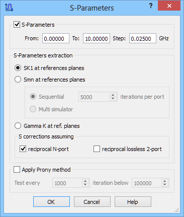
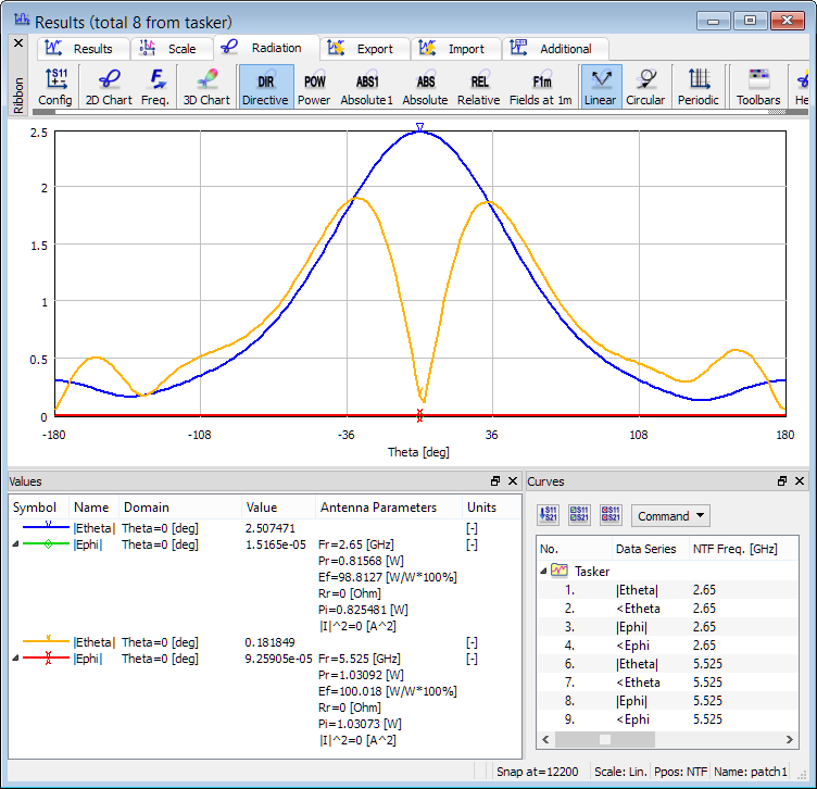
The S-Parameters postprocessing is set from 0 GHz to 10 GHz with the frequency step of 0.025 GHz.
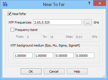
The radiation pattern calculations are set at 2.65 GHz and 5.525 GHz.
S-Parameters postprocessing and Near To Far postprocessing settings dialogues.
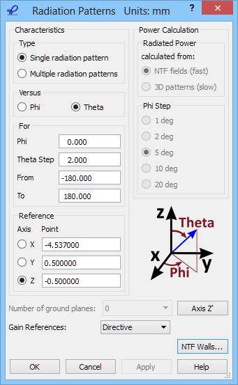
We wish to calculate the 2D radiation patterns versus angle Theta varying between -180 and 180 degrees with a step of 2 degrees. They will be calculated with a constant Phi angle equal to 0 degrees. The definition of the angles is explained in the lower right part of the 2D Radiation Patterns configuration dialogue. Note that this definition depends on the choice of the reference axis. The angle Theta is always counted from the reference axis (Z in the considered example). The angle Phi is always counted around it
2D Radiation Patterns configuration dialogue.
The reference axis can be set to X, Y or Z by clicking respective radio buttons in the Axis column of the dialogue. There is also an option to define an arbitrary reference axis. For an example of application of this option, please refer to the Two dipoles in free space excited in phase.
We can also set the reference point or in other words the origin of the coordinate system for the NTF transformation. The position of the reference point does not influence the absolute values of the radiation patterns (in lossless NTF background medium) but it does influence their phase characteristics. Moving the reference point can be helpful in a search for the antenna electrical centre. The reference point position is expressed in the same coordinates and units as those used in the project and defined in the user interface. To recall what units have been used, we can just take a look at the title bar of the window. In the considered example we see Units: mm.
2D radiation patterns calculated at 2.65 GHz and 5.525 GHz.
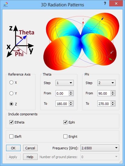
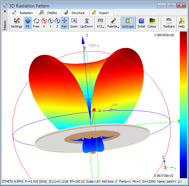
3D radiation pattern, with both Phi and Theta varying in steps, can be observed in the 3D Radiation Pattern window. The 3D Radiation Patterns configuration dialogue allows setting the reference axis and steps for angles Phi and Theta, defined with respect to that axis in the same way as for the 2D radiation pattern case. A single calculation frequency is also selected.
3D Radiation Patterns configuration dialogue.
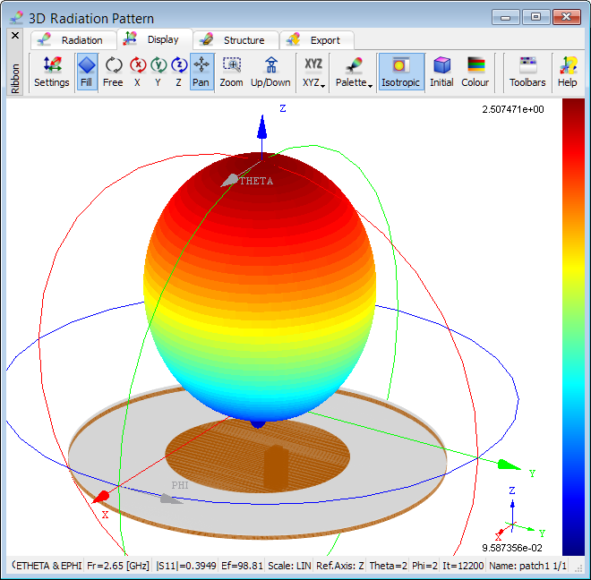
3D radiation pattern calculated at 2.65 GHz.
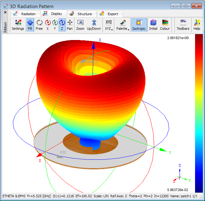
3D radiation pattern calculated at 5.525 GHz.