Rectangular waveguide to coaxial line transition
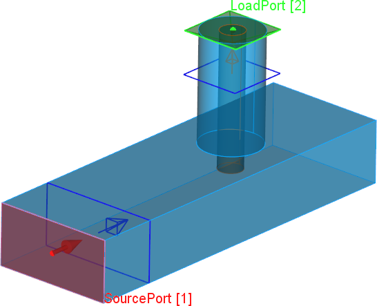
The present example considers a rectangular waveguide to coaxial line transition.
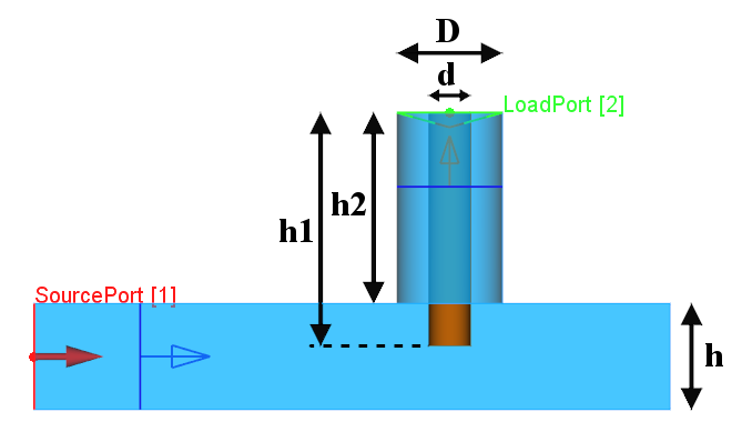
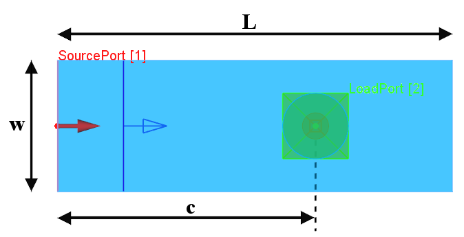
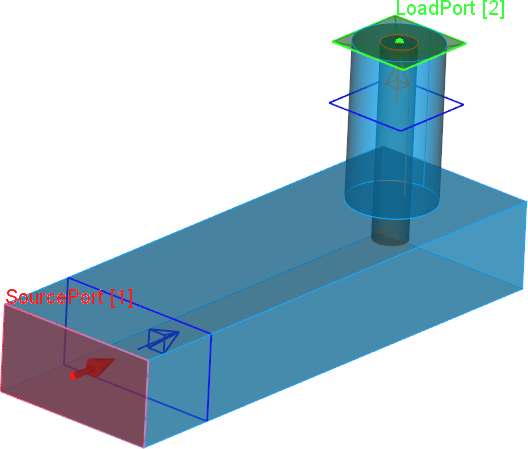
Rectangular waveguide to coaxial line transition scheme.
| Parameter |
w |
h |
L |
d |
D |
h1 |
h2 |
c |
| Value [mm] |
10 |
5 |
30 |
2 |
5 |
11 |
9 |
19.6 |
Rectangular waveguide to coaxial line transition parameters.
The input port is placed at the waveguide and it excites the fundamental TE10 mode and the output port with TEM mode is placed at the coaxial line.
Fundamental TE10 mode at the input port.
S-Parameters
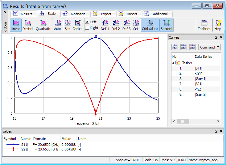
S-Parameters calculated for rectangular waveguide to coaxial line transition.
The obtained S-Parameters results indicated that our waveguide-to-coax transition is far from ideal design. There are relatively big reflections over most of the considered band and at the frequency f=20.65 GHz there is a total reflection. Before changing the design we may wish to know more about what caused such a reflection. Field distribution in the steady state at this frequency may be very helpful here. To obtain such a distribution we should change the waveform of the exciting signal to sinusoidal at 20.65 GHz.
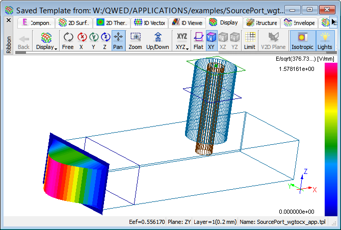
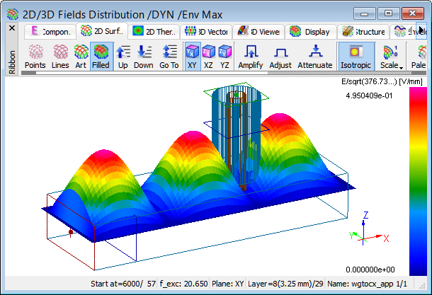
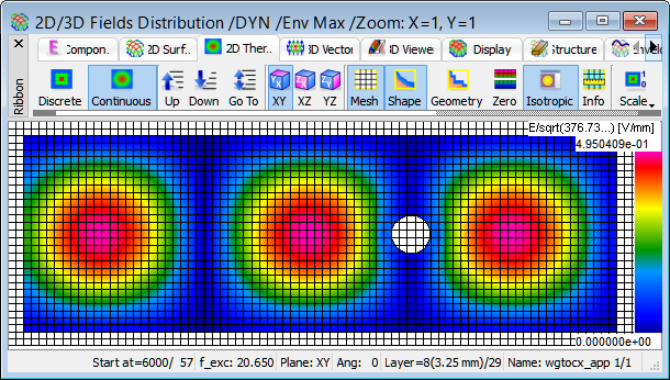
Display of Ez field in the envelope mode for the structure at 20.65 GHz.
Even a brief look at the envelope brings the conclusion that at the frequency 20.65 GHz we have a pure standing wave in the structure and that the reason for this standing wave is the transformation of the waveguide back short over a half-wavelength section to the coax output. Thus the coax output is effectively short-circuited and cannot receive energy from the waveguide. With the above conclusions we know that we need to modify the geometry of the transition and that we need to start by moving the coax output closer to the waveguide short.
Modified rectangular waveguide to coaxial line transition.
| Parameter |
w |
h |
L |
d |
D |
h1 |
h2 |
c |
| Value [mm] |
10 |
5 |
30 |
2 |
5 |
11.2 |
9 |
25 |
Rectangular waveguide to coaxial line transition modified parameters.
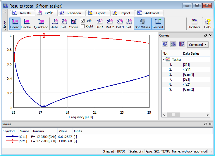
After modifying geometry parameters according to the table above, we run the simulation again (with original excitation pulse of spectrum f1<f<f2 with f1=15 GHz and f2=25 GHz). We can see that the performance of the transition has clearly improved and that, for example, we have reflections close to zero at 17.25 GHz.
S-Parameters calculated for modified rectangular waveguide to coaxial line transition.
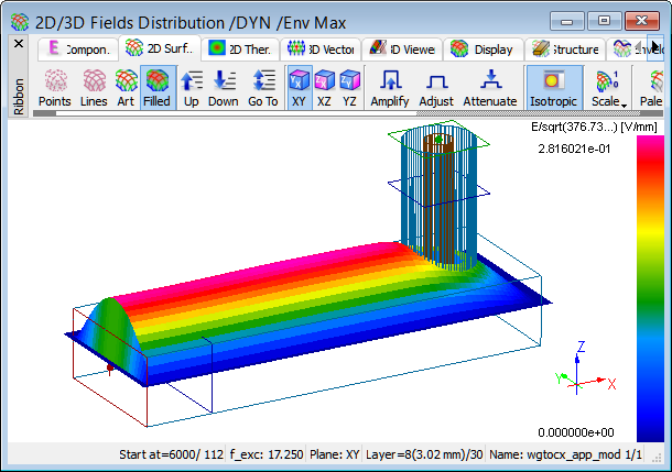
Let us now try to run the simulation of the modified structure with a sinusoidal excitation at aforementioned frequency. We obtain the image illustrating a purely travelling wave, which at the waveguide input is not perturbed by any reflections.
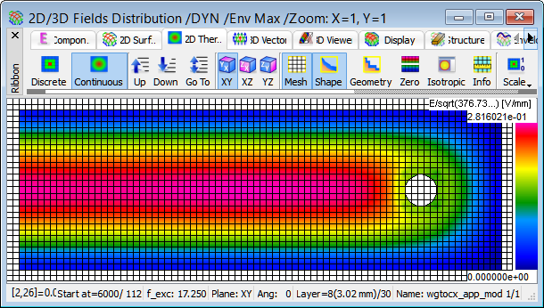
Display of Ez field in the envelope mode for the modified structure at 17.25 GHz.
S-Parameters below the cutoff frequency
We will now excite the structure with a wider frequency band from 10 GHz to 30 GHz. With a wider frequency band we excite the circuit at a higher resonant frequency (about 27 GHz) and also below the waveguide cutoff. Both excite slowly decaying processes and make the convergence to the final characteristics slower.
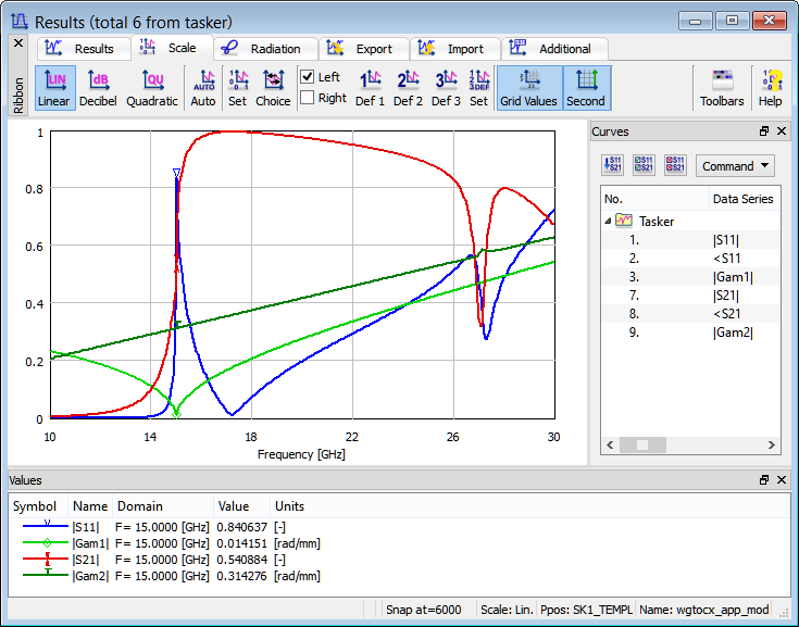
S-Parameters calculated for modified rectangular waveguide to coaxial line transition in a wider frequency band from 10 to 30 GHz.
|Gam1| and |Gam2| denote the absolute values of propagation constants in the transmission lines terminated by ports 1 and 2, respectively. It can be seen that at port 1 (waveguide input) the propagation constant drops to 0 at the waveguide cutoff (15 GHz), while at the TEM output |Gam2| is naturally proportional to the frequency.
Let us have a closer look at the values of |S11| and |S21| below the cutoff frequency. Naturally |S21| drops fast with decrease of the frequency. But what may seem less intuitive, there is also a fast decrease of |S11|. This is because even below the cutoff a long section of waveguide is reflectionless and thus its |S11| must tend to zero with the length of the section increasing. Let us also note that zero reflection does not imply any transmission of a real power into the guide since the characteristic impedance of the guide (equal to the reference impedance for S-parameter definition) is imaginary below the cutoff frequency.
The list of all parameters that can be calculated below cutoff frequency is given in Below cutoff calculations.
Extended S-Parameters
In some specific applications the user may require additional information about the phase angle of the propagation constant and about the changes in the characteristic impedances of the port lines (which are also reference impedances for the calculated S-matrix). To extract this extended information we need to activate Extended Results.
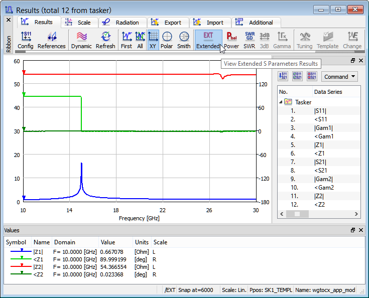
Extended S-Parameters calculated for modified rectangular waveguide to coaxial line transition in a wider frequency band from 10 to 30 GHz.
Taking advantage of this functionality, let us note for this considered case (see results above) that at the TEM output we have a constant and real impedance in the entire frequency band. At the waveguide input the impedance is real (<Z1=0) above the cutoff and imaginary (<Z1=90o) below the cutoff. The absolute value of the impedance changes in a way typical to a hollow waveguide TE mode that is, it rises when approaching the cutoff frequency. It is well known that a characteristic impedance of a waveguide is not uniquely definable and it is a subject of arbitrary normalisation. In QuickWave we normalize the characteristic impedance of a waveguide mode in such a way that it is equal to unity at the frequency at which the mode template has been calculated. In the considered example the input mode template has been calculated at 22.5 GHz and that is why |Z1|=1 at that frequency. Note however that in the case of TEM line for which the unique definition of impedance is possible, QuickWave indicates the actual impedance being Z2=54.4 Ω in our case.
Virtual shift of the reference plane
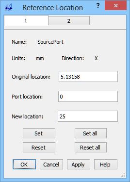
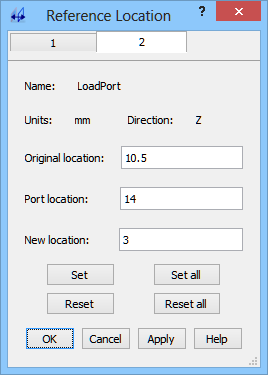
S-Parameters are extracted with respect to reference planes situated at some distance from the ports and that we can virtually move during results calculation. Let us now try to move the virtual reference planes of both ports to the position of the coaxial line antenna inserted into the waveguide. Thus we set in Port 1 New location=25 and in Port 2 New Location=3.
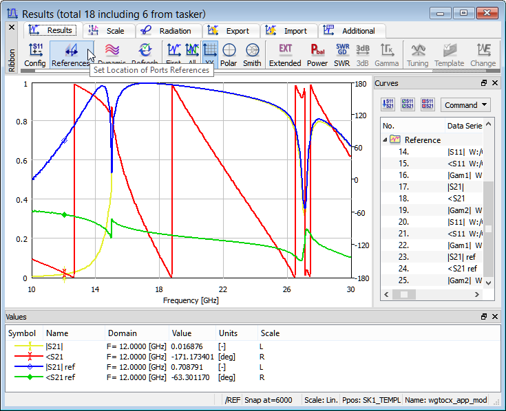
S-Parameters with the original reference planes (yellow + red) and the reference planes virtually moved to the position of the coax antenna (blue + green).
As expected, moving the reference plane makes the phase characteristics more flat (green line versus red line) and does not change |S21| above the waveguide cutoff (where the yellow line is hidden under the blue line). It is interesting to note that the software takes into account the real part of the propagation constant below the cutoff and appropriately corrects |S21| for low frequencies. That is why for example for 12 GHz |S21| rises from 0.0169 to 0.709.
Power Balance
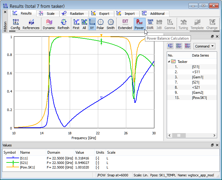
The power balance of the analysed structure can be activated with Power option in Results window. From the results shown below we can see that the list of the available curves offers either Pow.SK1 or Pow.Bal. to be displayed, with Extended Results off and on, respectively.
Power balance characteristic with standard (non-extended) S-Parameters.
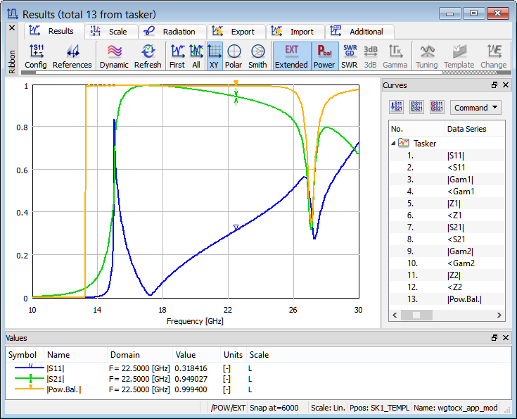
Power balance characteristic with extended S-Parameters.
In the case of extended S-Parameters the software calculates the actual power passing through each of the ports (contained in the mode assigned to a particular port). In such a case the power balance shows a square root of the ratio of the power dissipated in the load (or loads, in the case of multiports) to the power actually injected into the circuit from Port 1 working as the input. When Port 1 is unmatched or works below cut-off, the injected power may drop to zero. To avoid ill-conditioned calculations, Pow.Bal is set to zero when the injected power drops below 0.001 W threshold. It is recommended to refer to Power Balance for more details on power balance calculation and interpretation.
Full S-Matrix
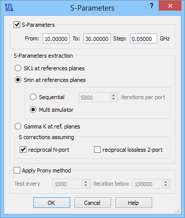
The entire S-matrix can be calculated using Smn at reference planes option in the S-Parameters postprocessing.
There are two computation regimes for full S-matrix calculations: Sequential and Multi simulator. The Sequential option means that is the considered case the software will first calculate S11 and S21 after excitation from Port 1 and simulation over the declared number of FDTD iterations. Then it will excite the structure from Port 2 and calculate S12 and S22. At the end it will perform matrix operations to correct mutually the results obtained with excitation from each port, and display the final result.
In the Multi simulator case the software will create two simulators being objects within QW-Simulator. Note that QW-Simulator has been developed in such a way that many simulator objects can exist and operate concurrently. In this case, one simulator will be running the FDTD analysis with excitation applied from Port 1, and thus extracting S11 and S21. The other simulator will be running the FDTD analysis with excitation applied from Port 2, and thus extracting S22 and S12. The Smn postprocessing functions will be importing data from both simulators on-line, and also on-line performing mutual corrections. Therefore the intermediate results watched during the analysis will already be mutually corrected; this is an important advantage with respect to the sequential mode where only the final result is mutually corrected. The other advantage is that the number of iterations per port does not have to be predefined, and the decision about terminating the analysis is made dynamically by the user as in the case of single-port excitation. However, memory occupation increases by a factor of two, which is a disadvantage in the case of analysing large problems on low-memory computers. The computing time remains unchanged: although the total number of iterations is reduced by a factor of two, the number of operations per iteration is doubled.
S-Parameters postprocessings settings dialogue.
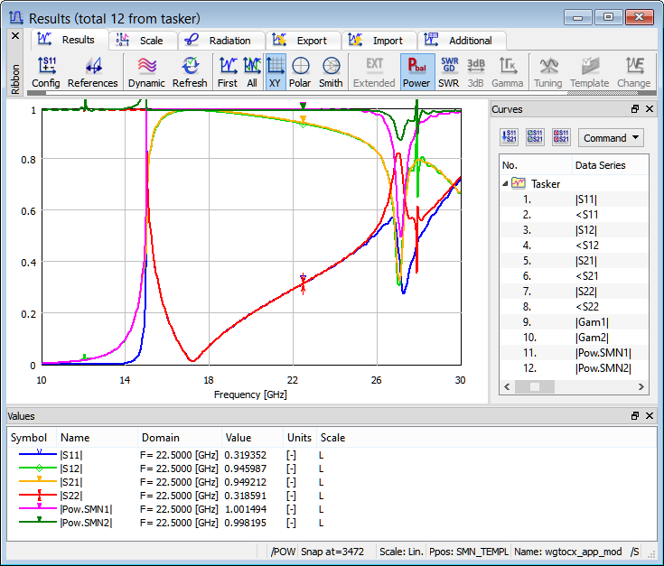
Results of full S-Matrix calculation contain 12 items, including all S-Matrix parameters, two propagation constants, and two power balance curves obtained with excitation from Port 1 and Port 2.
The obtained results show that in the entire frequency band |S21|=|S12|, which is a direct consequence of the circuit reciprocity. Moreover, in the band between 15 GHz and 25 GHz we also have |S11|=|S22|. The latter relation is due to the fact that in this band the circuit is a lossless reciprocal two-port with real reference impedances. Above 25 GHz some of the energy is leaking into the waveguide mode in the coaxial line like thus creating a kind of "losses" from the viewpoint of a two-port structure. Below 15 GHz the input reference impedance becomes imaginary and thus the relation |S11|=|S22| does not hold even for a lossless reciprocal two-port (as explained in the ref. [44]).