The radiation and scattering calculations deliver the following data:
Radiation patterns
QuickWave allows calculating radiation patterns of radiating structures using the Near to Far (NTF) post-processing. For radiation pattern calculation the so-called Huygens surface is required. This is the surface of the near-to-far field transformation, called in brief NTF Box, whereat the tangential near fields directly produced by the FDTD simulation are transformed into the far field radiation patterns using Green’s function.
NTF post-processing performs the near-to-far field transformation in the frequency domain to calculate the radiation patterns of a radiating structure, at frequencies specified by the user.
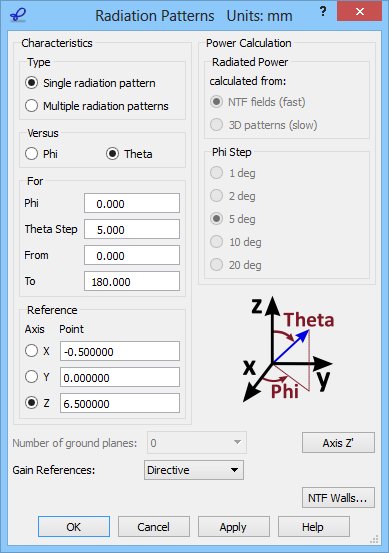
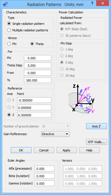
The far fields are available for any directions in space, with Reference Axis, Reference Point, angles and gain scaling options available for user's modifications. The far field patterns are calculated in a spherical coordinate system with one Reference Axis and two angles: elevation (Theta) and azimuthal (Phi).
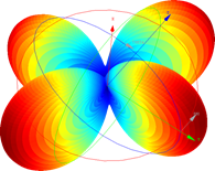
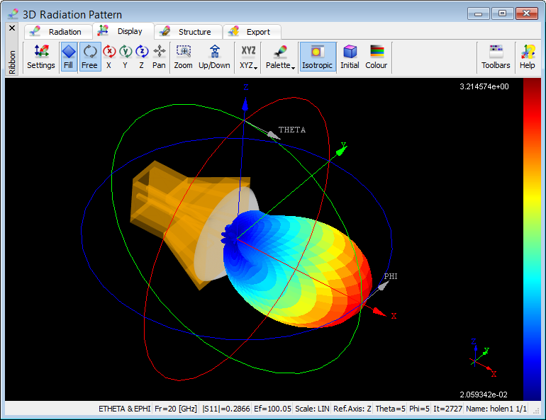
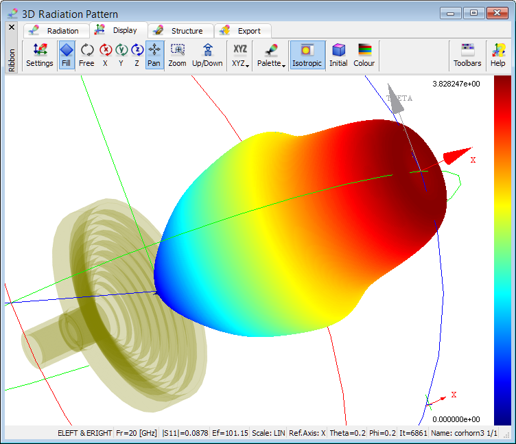
Far Field 3D radiation pattern
QucikWave enables calculation of 3D radiation pattern in a spherical coordinate system with one Reference Axis (X, Y or Z), two angles: elevation (Theta) and azimuthal (Phi) and for chosen NTF Frequency. The 3D radiation pattern may be constructed to show magnitudes of only Etheta, only Ephi or a vectorial sum of both, or only Eleft, only Eright or a vectorial sum of both.
Scattering patterns
QuickWave allows calculating far field scattering patterns of scattering structures irradiated by a free space incident wave, using the Near to Far (NTF) post-processing. For scattering pattern calculation the so-called Huygens surface is required. This is the surface of the near-to-far field transformation (called in brief NTF box), whereat the tangential near fields directly produced by the FDTD simulation are transformed into the far field scattering patterns using Green’s function.
It is worth noting at this point that QuickWave enables calculation of the scattering patterns of periodic structures, analysed using periodic boundary conditions. For this kind of problems the software automatically calculates the directions of higher diffraction order beams.
Radiation pattern at chosen Huygens surface
The principle of near-to-far field transformation requires that the radiating structure is surrounded by a closed surface (NTF box), unless symmetries are explored.
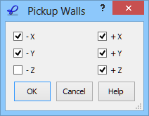
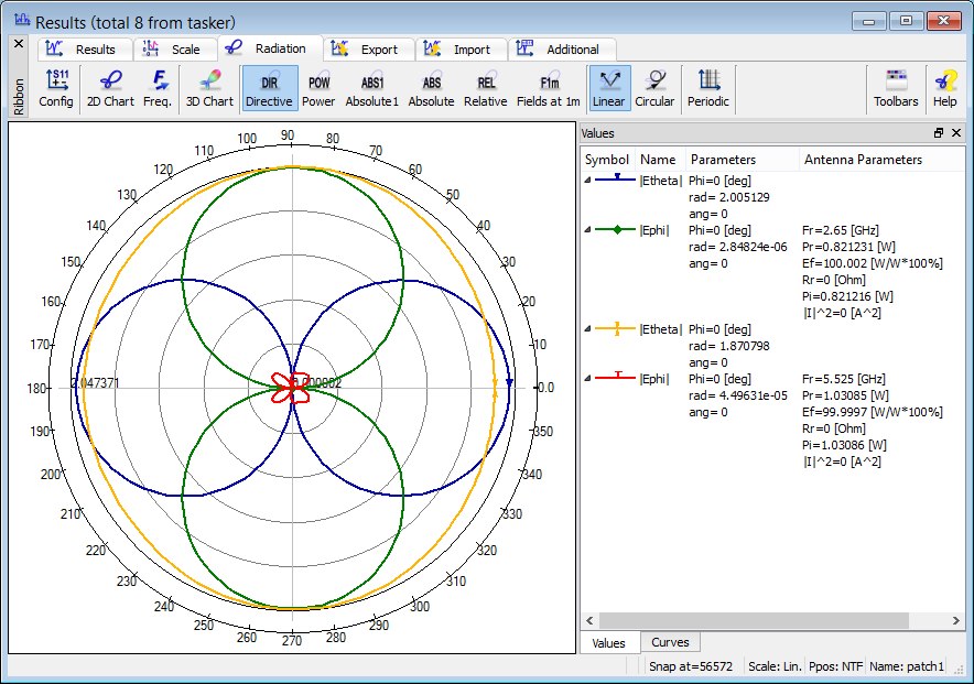
There are, however, cases when we may wish to calculate radiation patterns using only some of the NTF walls (pickup walls). A practical application would be to directly compare simulated and measured results, with near-field measurements taken over a single aperture. Another case is more FDTD-specific: due to numerical dispersion and the necessity to average either electric or magnetic field components across each pickup wall, a wave that physically propagates in one direction may numerically generate a non-physical backward lobe. A simple way to see whether a particular backlobe is physical or a numerical artefact is to disconnect the pickup surface "looking" in its direction from NTF transform and to check how the results change.
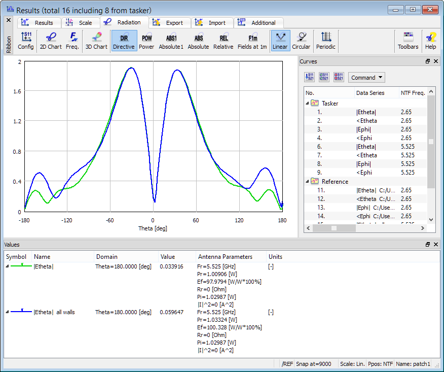
To exemplify this approach we consider the patch antenna example. The |Etheta| curve at 5.525 GHz has main beams around ±30o but also two weaker beams around ±160o. The user may wonder whether these are the actual downward propagating waves or numerical images of the upward ones.
To check whether EM energy is really radiated downwards by the considered patch, we exclude the bottom (–Z) wall from NTF transformation (the green curve). The ±160o lobes are reduced, compared to the complete NTF transform, and the green curve is practically monotone for large angles. This indicates that the patch does radiate through the –Z pickup wall. By comparing radiation efficiency and radiated power in the two cases we conclude that 2.34% of the total power radiated by the antenna exits the NTF box through the –Z wall.
Radiation pattern in an arbitrary isotropic medium
The near-to-far field transformation is usually applied in air, being the most typical environment for antennas. However, there are cases when transforming near fields to far fields in homogeneous media other than air or even lossy dielectrics is of interest. These may be biomedical applications or other cases of microwave propagation in large bodies. The air-formulation of NTF cannot be applied because impedance relation between the electric and magnetic field becomes different, and so does the propagation constant used in distance normalisation. NTF post-processing in QuickWave has been extended in response to such needs.
The region in which the radiating object (and thus the NTF box) is placed must be homogeneous and may be filled with a medium of arbitrary permittivity εr, permeability μr, conductivity σ and magnetic loss σm.
Antenna Gain
QuickWave offers several scaling options for antenna gain, which are available as Gain Reference option:
•
Directive – it refers to directive gain calculated with respect to the power radiated by the antenna. It is given as a unitless value.
•
Power – it equals to Directive gain multiplied by radiation efficiency in quadratic scale (i.e., in linear scale, Power gain equals to Directive gain multiplied by a square root of antenna efficiency).
•
Absolute_1port - it equals to Power gain multiplied by the coefficient of reflection loss (1-|S11|2) in quadratic scale (i.e., a square root of this coefficient in linear scale).
•
Absolute – it is calculated similarly to the Directive gain with this difference that here the power available from the source is taken as a reference.
•
Relative – it is calculated through normalisation to the highest value of the displayed pattern (except for cross-polarisation patterns normalised to the highest values of the corresponding co-polarisation patterns).
•
Fields at 1m – it refers to radiated field in the far zone scaled to 1m distance from the reference point using exp(-α*r)/r far field dependence.
Radiated Power
QuickWave calculates the total power radiated (Pr) from the antenna at given NTF frequencies. It is a time-maximum power radiated and it is used for gain calculation. The total radiated power is calculated only if the NTF post-processing is active and it is obtained through the integration operation. There are two options for radiated power calculations, corresponding directly to the radiation pattern calculation regime: integration in the near zone and integration in the far zone.
Radiation Efficiency
In case of antennas, the influence of losses on circuit performance is quantitatively described by radiation efficiency (Ef). The antenna radiation efficiency is calculated for NTF post-processing and is defined as the ratio of the radiated power (Pr) to the power injected into the antenna by the source (Pi).
Radiation Resistance
QuickWave delivers a value of antenna radiation resistance (Rr) at a given NTF frequency. Radiation resistance is defined as a ratio of radiated power (Pr) to the square of amplitude of current injected into the antenna by a point source.
Power injected by source
QuickWave delivers a value of the time-maximum power injected into antenna by the source (Pi) at a given NTF frequency. The value of Pi is calculated only if the S-Parameters post-processing at a source is active and one of its frequencies coincides with the given NTF frequency. Only with the S Parameters post-processing active the software has enough information to calculate the actual power injected by the source.
Current injected by source
QuickWave delivers a value of square of the amplitude of current injected into the antenna by a point source (|I|2) at a given NTF frequency. The value of |I|2 is calculated only if the FD-Probing post-processing at a point source is active and one of its frequencies coincides with the given NTF frequency. If there is no lumped source feeding antenna, the amplitude of the current injected into the antenna will not be calculated and its value will be 0.
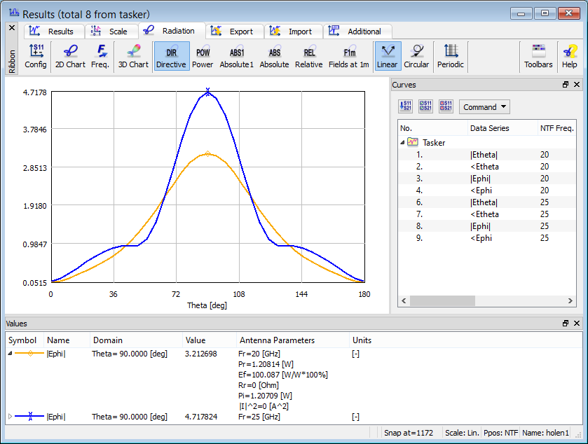
Linear Polarisation
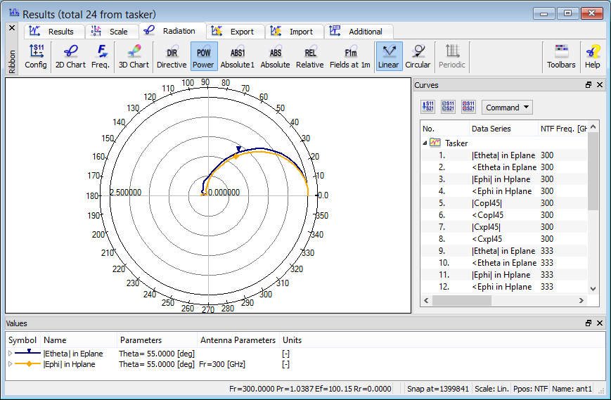
QuickWave extracts the radiation patterns in linear polarisation. Polarisation definition is based on the direction of the E-field with respect to the angular components Phi and Theta, thus for the linear polarisation, Etheta and Ephi curves are extracted.
In QW-V2D, for linear polarisation such results as Copl (co- polarisation) and Cxpl (cross polarisation) are additionally available.
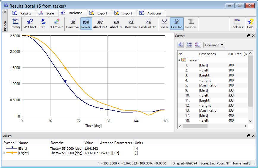
Circular Polarisation
Except for extracting radiation patterns in linear polarisation (Etheta and Ephi curves), it is also possible to switch to circular polarisation (Eleft and Eright curves). The convention for the left-handed Eleft and right-handed Eright circular polarisation is that for the outgoing wave.
If the analysed antenna is linearly polarised (one of Etheta or Ephi components is obviously dominant and the other is zero), the left- and right-handed polarisation curves practically overlap.
If the Etheta and Ephi curves are equal in magnitude and phase-shifted by 90 degrees, upon switching to circular polarisation circularly polarised wave will be observed with Eleft or Eright component being dominant.
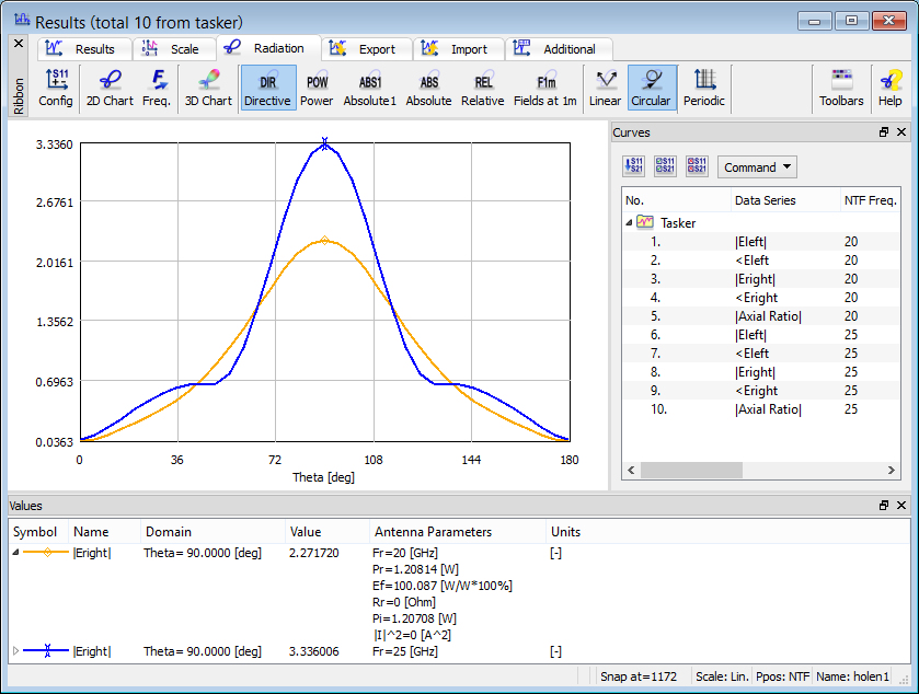
Axial Ratio
QuickWave calculates the Axial Ratio curves for antenna analysis. Axial ratio delivers information about the polarisation of the antenna since it is calculated from the ratio of the polarisation ellipse’s axes. If Axial Ratio=1 the antenna polarisation is circular. If the antenna is linearly polarised, the Axial Ratio will be equal to 0.